This is an analysis of 205 emails sent out from July 2019 to September 2020. A detailed explanation of the methodology and dataset can be found in the Discussion portion of this doc.
Takeaways
- Weekdays are better than weekends
- Emails sent before 9am don’t perform very well
- Take advantage of MailChimp’s “Send with TimeWarp,” especially for morning emails
- For late afternoons, 5pm is better than 6pm
What’s the best day to send emails?
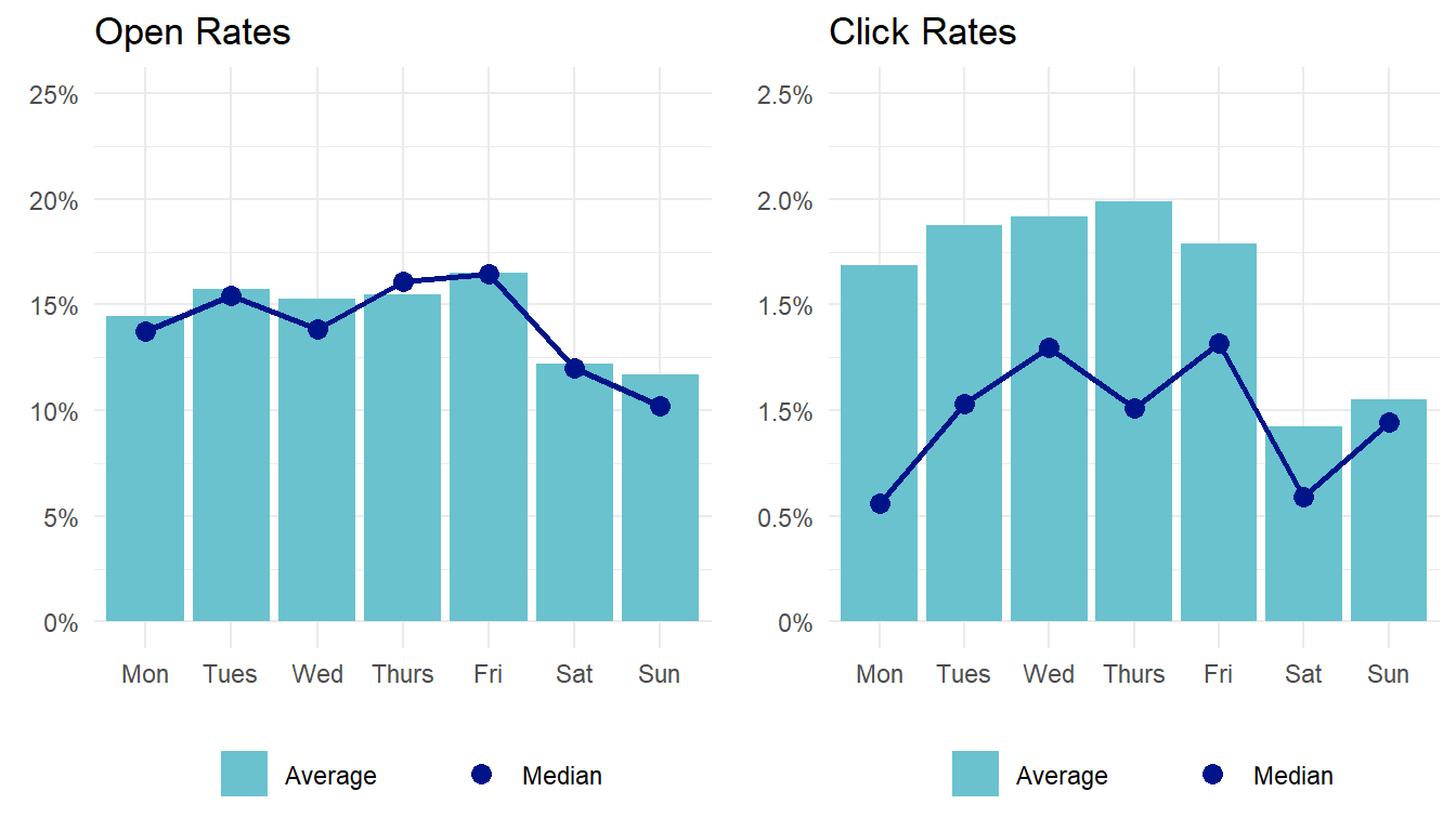
Generally speaking, weekdays are good, weekends aren’t, and Mondays seem to fall somewhere in between. There is some variation within weekdays - from the charts below, you can see that Friday open rates seem moderately better than Tuesday through Thursday, and that Mondays appear worse than other weekdays for both open and click rates.
But don’t read too much into that. There’s not enough certainty in these data to say that the distribution of the next 200 emails will be quite as favorable to Fridays and unfavorable to Mondays, and there’s too much noise in the click rate data to make any definitive statements at all. So the one solid conclusion that you can take to the bank - open rates are better on weekdays then on weekends.
What’s the best time to send emails?
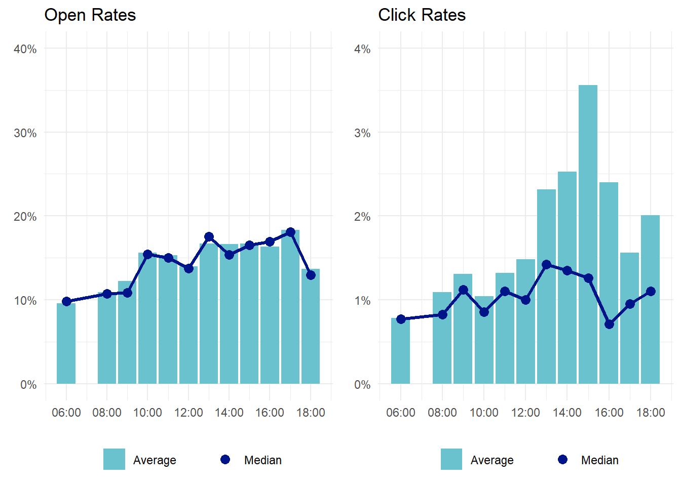
We have more categories for send time, which means fewer observations per category and therefore a little less certainty. But one thing we can say with relative certainty is that in terms of open rates, emails sent before 9am don’t perform very well. So for morning emails, take advantage of MailChimp’s “Send with Timewarp” option - this will deliver your campaign according to the recipient’s time zone, and avoid hitting any West Coast inboxes during the 6-8am window.
Note that 9am emails don’t appear to have great open rates - but we haven’t sent enough emails at that hour to firmly say that their poor performance is due to the timing rather than some other factor. If you google “what time should I send this email,” a lot of sites will recommend the 9am hour, so it wouldn’t be a bad idea to send a few more out and see how they do.
One additional interesting tidbit - there was a statistically significant difference between open rates for emails sent at 5pm and 6pm, with the 5pm emails outperforming the 6pm. The average click rates at 6pm are moderately higher, but the difference isn’t significant. So if you’re sending something late in the afternoon, shoot for 5 instead of 6.
There were a handful of emails sent at 7pm or later that aren’t included in the below plots since there are only one or two observations in each hour.
Discussion
The Sample
A few emails were removed from this dataset. First, those sent by users outside of the division, both because we have little control over when they are sent, and because their audience and purpose differ in scope from the emails that this discussion is intended to help inform. Second, all emails that included the word “COVID” in the email name. My assumption was that emails addressing the initial COVID-19 outbreak were sent in extremely abnormal circumstances, and therefore the results of those emails wouldn’t be generalizable to future emails. In an effort to introduce as little subjectivity as possible, all of these datapoints were removed before any analysis was performed.
One outlier was removed during the analysis portion of this project. For a full explanation, see the “Outlier” section below.
All email send times are rounded down to the nearest hour. I.e., an email sent at 9:47 would be categorized as a 9:00 email. This rounding was done based partly on the assumption that emails are typically targeted to be sent on the hour, partly on the assumption that most people operate on the hour. In other words, someone’s behavior at 11:45 is more likely to match what they’re doing at 11:00 (sitting at their desk) than at 12:00 (eating lunch). I contemplated breaking the data into half hour increments, but that would have created twice as many time categories resulting in a corresponding drop in certainty in our results. Additionally, I could have treated send time as a numerical rather than categorical variable. I opted for categorical/binned numerical primarily so that we could consider averages at given points throughout the day.
You might have noticed that I found basically no solid conclusions about the best day or time to send emails in regards to click rates. My best guess is that this is because the dataset includes both emails with a call to action and without. There was no easy way to parse these categories out, so I made no attempt to account for that variables. That means that an email with no call to action that gets a 0% click rate is seen as “bad,” even if that’s not really an accurate reflection of the email. The best solution to this will be better email naming convention practices going forward, which will help to separate out emails intended to receive clicks versus those that aren’t when considering click rates. But keep in mind that narrowing our scope will also narrow our sample size, which will make it more difficult to draw solid conclusions.
Variables
We’re looking at four variables: Day sent, time sent, open rate, and click rate. It’s useful to look at the distribution of each observation before diving into the analysis.
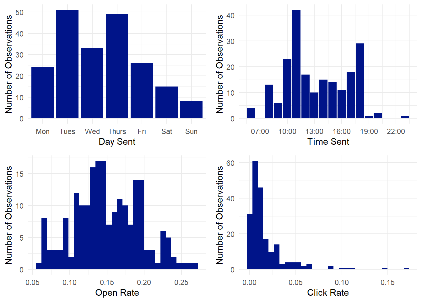
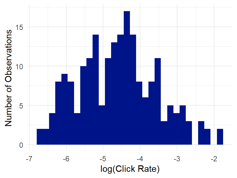
A couple of things jump out. First, a relatively low number of weekend emails was sent. Second, there aren’t a ton of observations in the 7pm and later categories, so we’ll remove those when analyzing send times since there’s not enough data there to draw solid conclusions. Third, the open rate distribution is relatively normal, which is good, because the ANOVA testing that we’ll do later assumes normality. But the click rates most definitely do not have a normal distribution, and are skewed pretty heavily to the right. Which is OK, because we can fix that with a simple logarithmic transformation:
Outlier Detection
A note on outliers - there are a lot of ways to define “outliers” and none of them are perfect. In general you shouldn’t remove an extreme data point from your data unless you have a really good reason to. A good reason might be that you think the result was recorded incorrectly or the datapoint is unique from the others in the data. A bad reason would be that the point changes your underlying assumptions about your data. If that’s the case, it says more about the rest of your data (largely that you don’t have enough of it) than it does about the one extreme point in question.
Open Rate
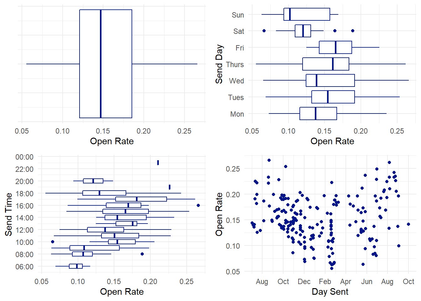
First, note the somewhat u-shaped distribution in the fourth plot. We’ll examine that a bit later, it’s kind of interesting.
From an outlier perspective, these data aren’t too concerning at all. There are a couple of odd ones on Saturdays that generally balance each other out. There are two extremes that are sent at odd times - those are removed from the top-line send time time data since they’re the only datapoints in those categories and don’t show us anything useful. The single .8 open rate is worth looking at –
| Details | Sent Date and Time | Day | Open_Rate | Click_Rate |
|---|---|---|---|---|
| Very Important and Unusual Email Title | 08/21/2019 16:32:00 | Wed | 0.265857 | 0.17139 |
There could be an argument to remove this point from the data - the content of this email is obviously more relevant than the time that it was sent. But let’s hold our judgement until we see whether or not that email was radically different from a clickrate perspective.
Last but not least, I said that the distribution looks normal. We can formalize that using the Shapiro-Wilk’s test for normality, which is testing
\(H_0\): Data are normally distributed
\(H_A\): Data are not normally distributed
##
##  Shapiro-Wilk normality test
##
## data:  dat$Open_Rate
## W = 0.99039, p-value = 0.1869
A p-value greater than 0.05 is not enough evidence to reject the null hypothesis, so we fail to reject and conclude that the data are normally distributed.
Click Rate
Going forward, we’re only concerned with the log transformation of our click rate, because the end goal is to perform an ANOVA analysis that assumes a multivariate normal distribution. You don’t need to be too concerned with what this means for interpreting the results. It doesn’t change how we’re going to interpret our send times or days, just how the formulas will interpret the click rates behind the scenes.
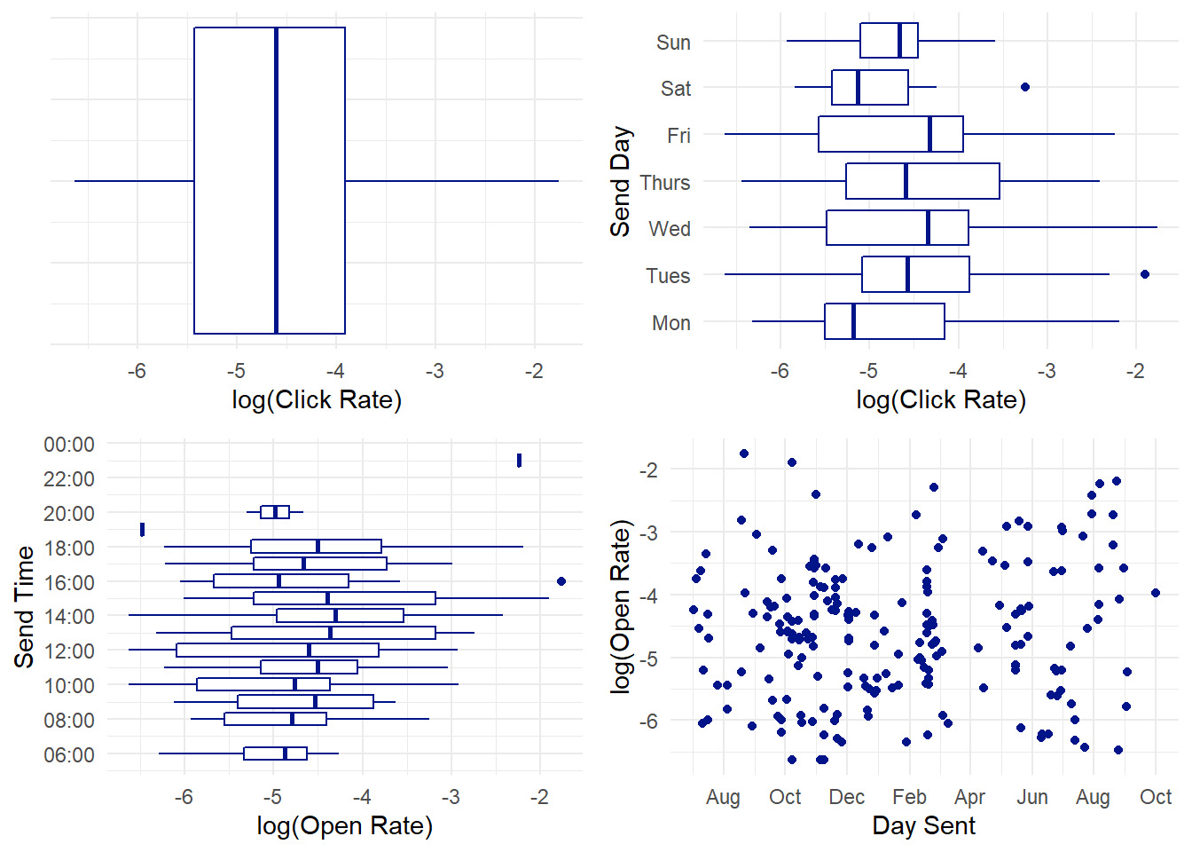
Overall the log transformation preempted a lot of outlier issues. There are two Tuesday extremes that look like they pretty much balance each other out. There’s one relatively high Saturday rate that we should look at. As mentioned above, we’re not going to pay too much attention to the emails sent at 7pm or later because there’s not enough data to make any solid conclusions. But the 16:00 (4pm) outlier is interesting.
| Details | Sent Date and Time | Day | Open_Rate | Click_Rate |
|---|---|---|---|---|
| Generic Email Title | 05/16/2020 14:37:00 | Sat | 0.1253041 | 0.0054745 |
| Very Important and Unusual Email Title | 08/21/2019 16:32:00 | Wed | 0.2658570 | 0.1713900 |
The generic email title, while interesting, isn’t going to change any of our ultimate conclusions, and the email itself isn’t that abnormal. But the super important email is popping up again as an extreme case. At this point I think we have sufficient evidence to remove it from our data due to it’s status as an outlier. Which we shouldn’t do lightly. If it were a more generic email I’d keep it in, but it’s pretty self-evident that the exceptional performance of this email was due more to the nature of the email than any magic behind when it was sent.
Hypothesis Testing
ANOVA
We’re first going to conduct a series of ANOVA analyses on our four relationships, which will test whether there is a significant difference in means between categorical variables. ANOVA stands for Analysis of Variance, and focuses on the variation in the data. To illustrate how it works, imagine that you sent 20 emails on Tuesdays, and every one of them had an open rate between .29 and .31. You could be pretty certain that your next Tuesday email would have have an open rate of about .30. Imagine you sent another 20 emails on Wednesdays, and they ranged from .09 to .51. The average is still .30, but you’re going to be much less confident that the next email you send will also have a .30 open rate. ANOVA is calculating that confidence, and taking it into account when considering whether the averages between days are really significantly different.
In every instance, we’re looking for a p-value less than 0.05 - that will suggest that the differences between groups are significant enough that we can conclude that they are due to our independent variables (date or time) rather than noise in the data.
Below are our hypothesis tests, the ANOVA results, and our conclusions:
Open Rates - Send Days
\(H_0\): There is no difference in open rates between days
\(H_A\): There is a difference in open rates between days
##              Df Sum Sq  Mean Sq F value Pr(>F)
## Day           6 0.0312 0.005193   2.728 0.0144 *
## Residuals   199 0.3789 0.001904
## ---
## Signif. codes:  0 '***' 0.001 '**' 0.01 '*' 0.05 '.' 0.1 ' ' 1
We have a p-value <0.05, so there is sufficient evidence to reject the null hypothesis and conclude that there is a statistically significant difference in open rates between days.
Open Rates - Send Times
\(H_0\): There is no difference in open rates between times
\(H_A\): There is a difference in open rates between times
##              Df Sum Sq  Mean Sq F value   Pr(>F)
## Time         14 0.0897 0.006409   3.822 1.04e-05 ***
## Residuals   191 0.3203 0.001677
## ---
## Signif. codes:  0 '***' 0.001 '**' 0.01 '*' 0.05 '.' 0.1 ' ' 1
We have a p-value <0.05, so there is sufficient evidence to reject the null hypothesis and conclude that there is a statistically significant difference in open rates between times.
Click Rates - Send Days
\(H_0\): There is no difference in click rates between days
\(H_A\): There is a difference in click rates between days
##              Df Sum Sq Mean Sq F value Pr(>F)
## Day           6   3.31  0.5521   0.488  0.817
## Residuals   199 224.96  1.1304
We have a p-value >0.05, so there is insufficient evidence to reject the null hypothesis. There is not enough evidence to conclude that there is a statistically significant difference in click rates between days.
Click Rates - Send Times
\(H_0\): There is no difference in click rates between times
\(H_A\): There is a difference in click rates between times
##              Df Sum Sq Mean Sq F value Pr(>F)
## Time         14  21.35   1.525   1.407  0.153
## Residuals   191 206.93   1.083
We have a p-value >0.05, so there is insufficient evidence to reject the null hypothesis. There is not enough evidence to conclude that there is a statistically significant difference in click rates between times.
Tukey’s Post-Hoc Analysis
Tukey’s Post-Hoc test looks at direct comparisons within groups - where the ANOVA test is looking for whether there is a significant difference between groups, Tukey’s Post-Hoc analysis asks the question, which groups? We’re only performing Tukey’s test on open rates, because the click rate relationships weren’t significant.
A smattering of the more significant differences (p <= 0.25) are below - but keep in mind that the only “statistically significant” difference are those with a p-value (furthest right column) of 0.05 or less. And if you want to engage in a discussion of why the concept of “statistically significant” is kind of arbitrary and a bit flawed, give me call.
| comparison | diff | lwr | upr | p adj |
|---|---|---|---|---|
| Sat-Tues | -0.0352746 | -0.0734520 | 0.0029028 | 0.0910293 |
| Sun-Tues | -0.0404160 | -0.0898427 | 0.0090106 | 0.1893898 |
| Sat-Thurs | -0.0328754 | -0.0712295 | 0.0054786 | 0.1464336 |
| Sat-Fri | -0.0433604 | -0.0855033 | -0.0012175 | 0.0392086 |
| Sun-Fri | -0.0485019 | -0.1010519 | 0.0040482 | 0.0917121 |
| comparison | diff | lwr | upr | p adj |
|---|---|---|---|---|
| 13:00-06:00 | 0.0710298 | -0.0122265 | 0.1542860 | 0.1916388 |
| 14:00-06:00 | 0.0706798 | -0.0085127 | 0.1498723 | 0.1384795 |
| 15:00-06:00 | 0.0709505 | -0.0088352 | 0.1507362 | 0.1423817 |
| 16:00-06:00 | 0.0674874 | -0.0146805 | 0.1496553 | 0.2441598 |
| 17:00-06:00 | 0.0873440 | 0.0095532 | 0.1651347 | 0.0126736 |
| 19:00-06:00 | 0.1307719 | -0.0265677 | 0.2881114 | 0.2270401 |
| 10:00-08:00 | 0.0471353 | -0.0016960 | 0.0959667 | 0.0708922 |
| 11:00-08:00 | 0.0443921 | -0.0002729 | 0.0890572 | 0.0532378 |
| 13:00-08:00 | 0.0579390 | -0.0012547 | 0.1171326 | 0.0620089 |
| 14:00-08:00 | 0.0575890 | 0.0042623 | 0.1109157 | 0.0209462 |
| 15:00-08:00 | 0.0578597 | 0.0036560 | 0.1120634 | 0.0241344 |
| 16:00-08:00 | 0.0543966 | -0.0032562 | 0.1120494 | 0.0873819 |
| 17:00-08:00 | 0.0742532 | 0.0230313 | 0.1254751 | 0.0001387 |
| 17:00-09:00 | 0.0606498 | -0.0056904 | 0.1269900 | 0.1144330 |
| 17:00-12:00 | 0.0431472 | -0.0044473 | 0.0907416 | 0.1225126 |
| 18:00-17:00 | -0.0464299 | -0.0886575 | -0.0042023 | 0.0167000 |
The ANOVA and Tukey tests for click rates excludes all categories with less than four observations. I quibbled on whether or not to exclude the 6am hour (four observations), but thought it was worth looking at since there is evidence to suggest we shouldn’t be sending at that time. But keep in mind that the sample size is small, and would warrant more testing.
A note on the odd February dip
These data are chronologically ordered, so the roughly u-shaped open rate distribution (below left) is a bit odd. We can see that the bottom of the distribution seems to be centered around February, which makes sense - there is a large campaign in February that sees emails to a very broad audience, and we would expect those emails to see a lower open rate than the generally more targeted emails. Let’s see what happens to our distribution when we remove any email with “Feb_Campaign” in the title (below right).
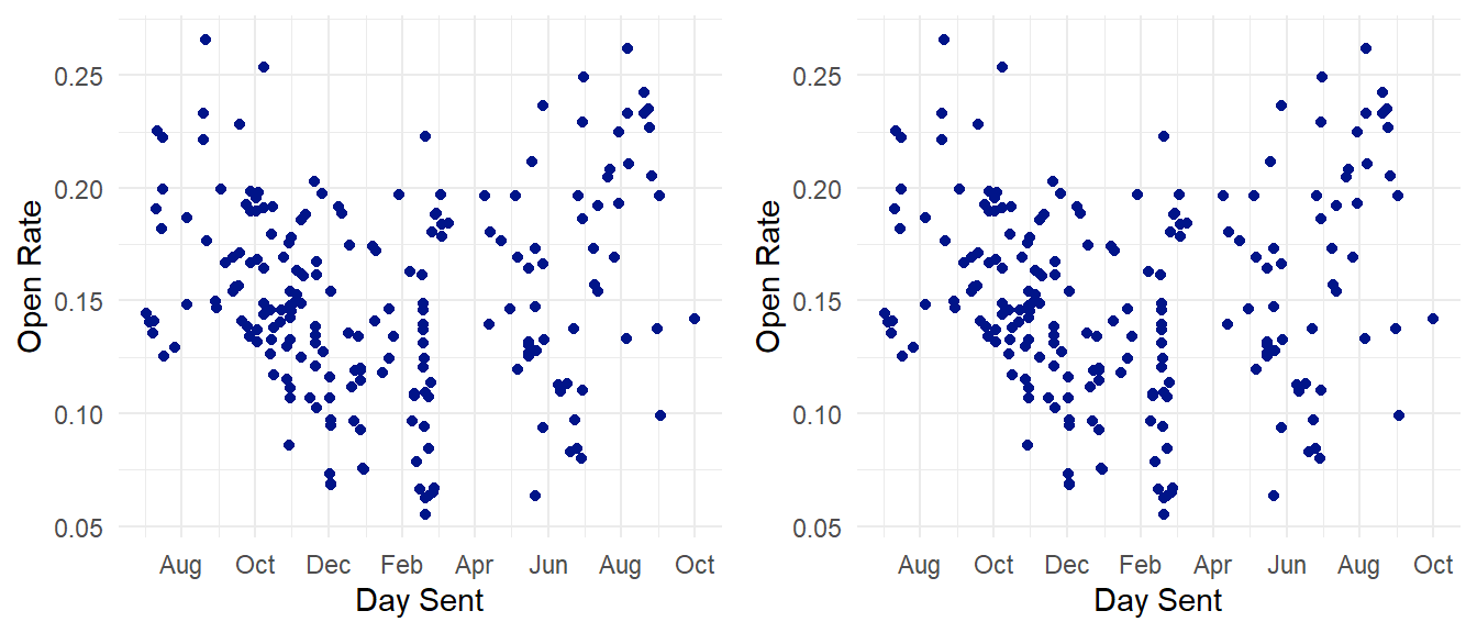
That definitely looks more normal. There are still some high-performing emails around the end of summer, but they’re not nearly as dramatic as the dip in February was. How much do the February Campaign emails affect our overall open rates?
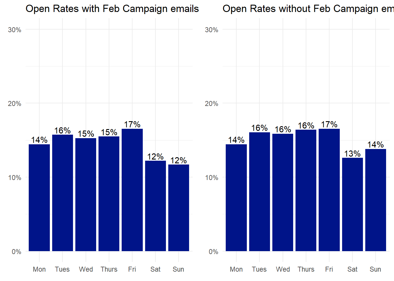
Actually not all that much. If anything, removing these data reinforces the point that Tuesdays through Fridays are better than weekends, and that the jury is still out on Mondays. Removing them doesn’t change the bottom line in any of our ANOVA analysis or Tukey’s followup.
Document Information
All of the statistical analyses in this document were performed using R version 4.0.2 (2020-06-22). R packages used will be maintained using the packrat dependency management system. For questions, data, or to view full code, contact Jon Crenshaw at jon.crenshaw@colby.edu
## R version 4.0.2 (2020-06-22)
## Platform: x86_64-w64-mingw32/x64 (64-bit)
## Running under: Windows 10 x64 (build 19041)
##
## Matrix products: default
##
## locale:
## [1] LC_COLLATE=English_United States.1252
## [2] LC_CTYPE=English_United States.1252
## [3] LC_MONETARY=English_United States.1252
## [4] LC_NUMERIC=C
## [5] LC_TIME=English_United States.1252
##
## attached base packages:
## [1] stats     graphics  grDevices utils     datasets  methods   base
##
## other attached packages:
##  [1] kableExtra_1.3.4 tibble_3.1.0     agricolae_1.3-3  tidyr_1.1.2
##  [5] fmsb_0.7.0       lubridate_1.7.10 mvnormtest_0.1-9 gridExtra_2.3
##  [9] scales_1.1.1     forcats_0.5.1    ggplot2_3.3.3    dplyr_1.0.4
## [13] readxl_1.3.1
##
## loaded via a namespace (and not attached):
##  [1] httr_1.4.2        sass_0.3.1        jsonlite_1.7.2    viridisLite_0.3.0
##  [5] bslib_0.2.4       shiny_1.6.0       highr_0.8         cellranger_1.1.0
##  [9] yaml_2.2.1        pillar_1.5.1      lattice_0.20-41   glue_1.4.2
## [13] digest_0.6.27     promises_1.2.0.1  rvest_0.3.6       colorspace_2.0-0
## [17] htmltools_0.5.1.1 httpuv_1.5.5      klaR_0.6-15       pkgconfig_2.0.3
## [21] labelled_2.7.0    haven_2.3.1       questionr_0.7.4   bookdown_0.21
## [25] purrr_0.3.4       xtable_1.8-4      webshot_0.5.2     svglite_2.0.0
## [29] later_1.1.0.1     combinat_0.0-8    farver_2.1.0      generics_0.1.0
## [33] ellipsis_0.3.1    withr_2.4.1       magrittr_2.0.1    crayon_1.4.1
## [37] mime_0.10         evaluate_0.14     fansi_0.4.2       nlme_3.1-148
## [41] MASS_7.3-51.6     xml2_1.3.2        blogdown_1.2      tools_4.0.2
## [45] hms_1.0.0         lifecycle_1.0.0   stringr_1.4.0     munsell_0.5.0
## [49] cluster_2.1.0     compiler_4.0.2    jquerylib_0.1.3   systemfonts_1.0.1
## [53] rlang_0.4.10      grid_4.0.2        rstudioapi_0.13   miniUI_0.1.1.1
## [57] labeling_0.4.2    rmarkdown_2.7     gtable_0.3.0      AlgDesign_1.2.0
## [61] R6_2.5.0          knitr_1.31        fastmap_1.1.0     utf8_1.1.4
## [65] stringi_1.5.3     Rcpp_1.0.6        vctrs_0.3.6       tidyselect_1.1.0
## [69] xfun_0.21